Spatial Data Wrangling (2) – GIS Operations
Original GeoDa lab by Luc Anselin: https://geodacenter.github.io/workbook/01_datawrangling_2/lab1b.html
Introduction
Even though Kepler.gl and GeoDa are not GIS by design, a range of spatial data manipulation functions are available that perform some specialized GIS operations. This includes an efficient treatment of projections, conversion between points and polygons, the computation of a minimum spanning tree, and spatial aggregation and spatial join through multi-layer support.
Objectives
- Understand how projections are expressed in a coordinate reference system (CRS)
Be able to efficiently change from one projection to another- Create shape centers (mean center and centroid) for polygons
- Construct Thiessen polygons for a point layer
- Compute a minimum spanning tree based on the max-min distance between points
- Dissolve areal units and compute aggregate values
- Compute aggregate values based on a common indicator in a table
- Operate on more than one layer
- Implement a spatial join to carry out point in polygon operations
Visualize the common link between two layers
Preliminaries
We will continue to illustrate the various operations by means of a series of example data sets, all contained in the GeoDa Center data set collection.
Some of these are the same files used in the previous chapter. For the sake of completeness, we list all the sample data sets used:
Chicago commpop: population data for 77 Chicago Community Areas in 2000 and 2010 https://geodacenter.github.io/data-and-lab/data/chicago_commpop.geojson
Groceries: the location of 148 supermarkets in Chicago in 2015 https://geodacenter.github.io/data-and-lab//data/chicago_sup.geojson
Natregimes: homicide and socio-economic data for 3085 U.S. counties in 1960-1990 https://geodacenter.github.io/data-and-lab/data/natregimes.geojson
Home Sales: home sales in King County, WA during 2014-2015 (point data) https://geodacenter.github.io/data-and-lab//data/KingCountyHouseSales2015.geojson
Projections
Spatial observations need to be georeferenced, i.e., associated with specific geometric objects for which the location is represented in a two-dimensional Cartesian coordinate system. Since all observations originate on the surface of the three-dimensional near-spherical earth, this requires a transformation. The transformation involves two steps that are often confused by non-geographers. The topic is complex and forms the basis for the discipline of geodesy. A detailed treatment is beyond our scope, but a good understanding of the fundamental concepts is important. The classic reference is Snyder (1993), and a recent overview of a range of technical issues is offered in Kessler and Battersby (2019).
The basic building blocks are degrees latitude and longitude that situate each location with respect to the equator and the Greenwich Meridian (near London, England). Longitude is the horizontal dimension (x), and is measured in degrees East (positive) and West (negative) of Greenwich, ranging from 0 to 180 degrees. Since the U.S. is west of Greenwich, the longitude for U.S. locations is negative. Latitude is the vertical dimension (y), and is measured in degrees North (positive) and South (negative) of the equator, ranging from 0 to 90 degrees. Since the U.S. is in the northern hemisphere, its latitude values will be positive.
In Kepler.gl, the WGS84 geographic coordinate system is used by default. All data is visualized using latitude and longitude in this system to represent geographic locations accurately. Note: the GeoJSON format uses the WGS84 geographic coordinate system by default. If you have datasets not in the WGS84 geographic coordinate system, you can convert them to WGS84 using GeoDa software (see Reprojection).
However, when computing geometric measurements—such as distance, buffer, area, length, and perimeter—the AI assistant automatically uses GeoDa library to convert geographic coordinates (latitude and longitude) into projected coordinates (easting and northing) using the UTM projection with the WGS84 datum. This ensures accurate calculations in meters.
For Universal Transverse Mercator or UTM, the global map is divided into parallel zones, as shown in Figure below. With each zone corresponds a specific projection that can be used to convert geographic coordinates (latitude and longitude) into projected coordinates (easting and northing).
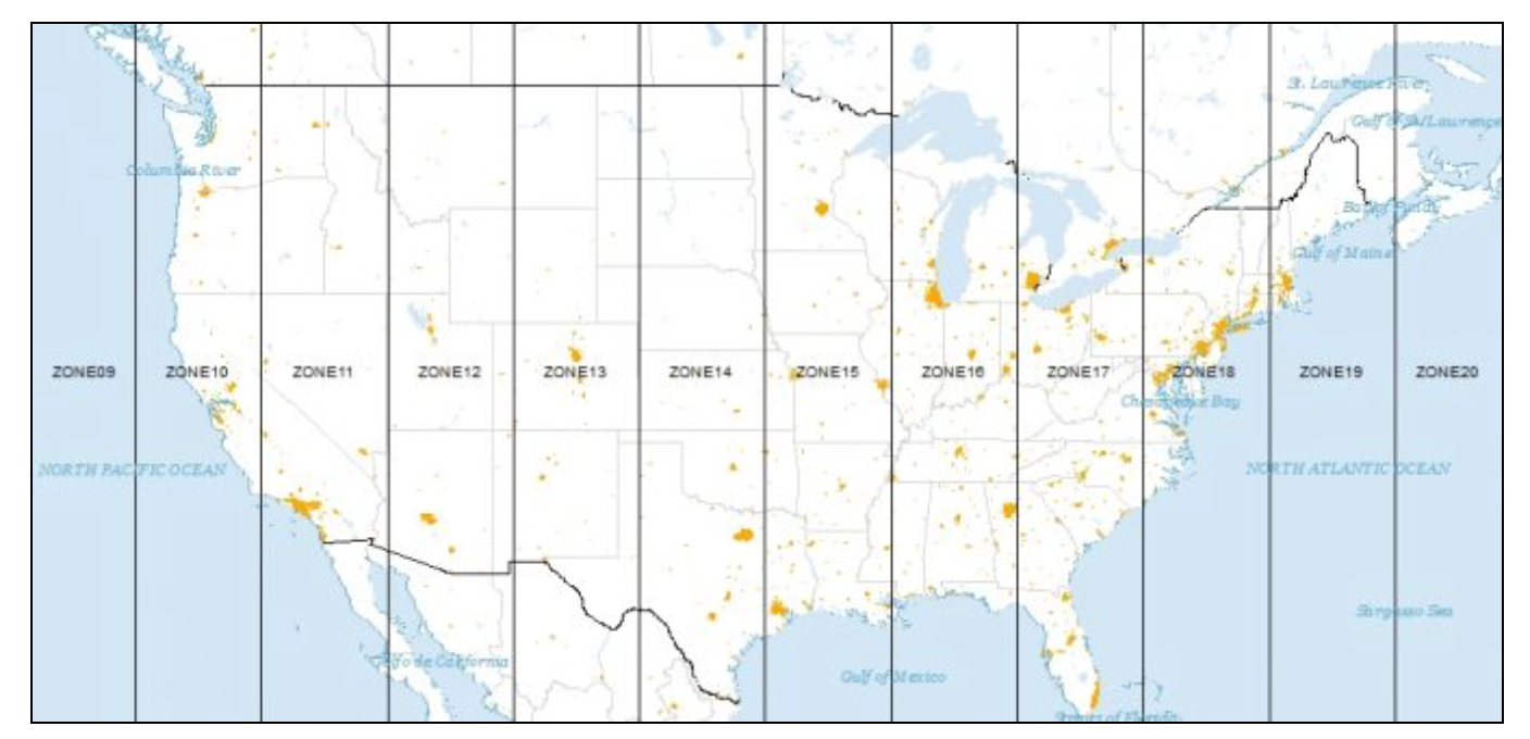 UTM zones for North America (source: GISGeography)
 Converting Between Points and Polygons
So far, we have represented the geography of the community areas by their actual boundaries. However, this is not the only possible way. We can equally well choose a representative point for each area, such as a mean center or a centroid. In addition, we can create new polygons to represent the community areas as tessellations around those central points, such as Thiessen polygons. The key factor is that all three representations are connected to the same cross-sectional data set. As we will see in later chapters, for some types of analyses it is advantageous to treat the areal units as points, whereas in other situations Thiessen polygons form a useful alternative to dealing with an actual point layer.
The center point and Thiessen polygon functionality is brought up through the options menu associated with any map view (right click on the map to bring up the menu). We illustrate these features with the projected community area map we just created.
Mean centers and centroids
The mean centers is obtained as the simple average of the the X and Y coordinates that define the vertices of the polygon. The centroid is more complex, and is the actual center of mass of the polygon (image a cardboard cutout of the polygon, the centroid is the central point where a pin would hold up the cutout in a stable equilibrium).
Both methods can yield strange results when the polygons are highly irregular or in a so-called multi-polygon situation (different polygons associated with the same ID, such as a mainland area and an island belonging to the same county). In those instances the centers can end up being located outside the polygon. Nevertheless, the shape centers are a handy way to convert a polygon layer to a corresponding point layer with the same underlying geography. For example, as we will see in a later chapter, they are used under the hood to calculate distance-based spatial weights for polygons.
To add centroids of the map layer, you can use the following prompt to create a map layer first:
Can you create a map layer from https://geodacenter.github.io/data-and-lab/data/chicago_commpop.geojson?After the map layer is created, you can add centroids by just prompting:
Can you get the centroids from the chicago commpop dataset?Thiessen polygons
Point layers can be turned into a so-called tessellation or regular tiling of polygons centered around the points. Thiessen polygons are those polygons that define an area that is closer to the central point than to any other point. In other words, the polygon contains all possible locations that are nearest neighbors to the central point, rather than to any other point in the data set. The polygons are constructed by considering a line perpendicular at the midpoint to a line connecting the central point to its neighbors.
For example, we can prompt the AI assistant to create Thiessen polygons for the point layer:
Can you create Thiessen polygons for the centroids?Minimum spanning tree
A graph is a data structure that consists of nodes and vertices connecting these nodes. In our later discussions, we will often encounter a connectivity graph, which shows the observations that are connected for a given distance band. The connected points are separated by a distance that is smaller than the specified distance band.
An important graph is the so-called max-min connectivity graph, which shows the connectedness structure among points for the smallest distance band that guarantees that each point has at least one other point it is connected to.
A minimum spanning tree (MST) associated with a graph is a path through the graph that ensures that each node is visited once and which achieves a minimum cost objective. A typical application is to minimize the total distance traveled through the path. The MST is employed in a range of methods, particularly clustering algorithms.
The Ai assistant uses GeoDa library to construct an MST based on the max-min connectivity graph for any point layer. The construction of the MST employs Prim’s algorithm, which is illustrated in more detail in the Appendix.
To create a minimum spanning tree for the point layer, you can use the following prompt:
Can you create a minimum spanning tree from the centroids?Aggregation
Spatial data sets often contain identifiers of larger encompassing units, such as states for counties, or census tracts for individual household data. Spatial disolve is a function that allows us to aggregate the smaller units into the larger units.
We illustrate this functionality with the natregimes dataset using spatial dissolve tool. First, load the dataset:
Load the dataset https://geodacenter.github.io/data-and-lab/data/natregimes.geojsonWhile the observations are for counties, each county also includes a numeric code for the encompassing state in the variable STFIPS. We can use this variable to aggregate the counties into states.
Can you aggregate the counties into states based on the STFIPS variable?If you want to aggregate the properties values of the counties into the states, you can use the following prompt:
Can you aggregate the counties into the states based on the STFIPS and aggregate the numeric variables by SUM?Multi-Layer Support
Kepler.gl supports multi-layer visualization by default. When you load more datasets, the map layers will be automatically added to current map. You can drag-n-drop the layers to reorder them. This multi-layer infrastructure allows for the calculation of variables for one layer, based on the observations in a different layer.
Load the dataset https://geodacenter.github.io/data-and-lab/data/chicago_commpop.geojsonLoad the dataset https://geodacenter.github.io/data-and-lab/data/chicago_sup.geojsonSpatial Join
This is an example of a point in polygon GIS operation. There are two applications of this process. In one, the ID variable (or any other variable) of a spatial area is assigned to each point that is within the area’s boundary. We refer to this as Spatial Assign. The reverse of this process is to count (or otherwise aggregate) the number of points that are within a given area. We refer to this as Spatial Count.
Even though the default application is simply assigning an ID or counting the number of points, more complex assignments and aggregations are possible as well. For example, rather than just counting the point, an aggregate over the points can be computed for a given variable, such as the mean, median, standard deviation, or sum. This process is called Spatial Join.
Spatial assign
We start the process illustrating the Spatial Assign operation by first loading the Chicago supermarkets point layer, chicago_sup.geojson, followed by the projected community area layer, chicago_commpop.geojson.
The purpose of the Spatial Assign operation is to assign the community area ID to each supermarket. This is done by using the Spatial Join tool.
Can you assign the community name to each supermarket in chicago_sup.geojson?Spatial count
The Spatial Count process works in the reverse order by counting the number of supermarkets in each community area.
Can you spatial join the points to the community areas and count the number of points in each community area?TIP
You can click on the spatialJoin tool to see the details of how spatial join tool has been applied on the datasets.
Spatial join with aggregation
We can also carry out an aggregation over the points in each area. For example, when joining the points to the community areas, we can aggregate the points by the mean of the variable NEAR_DIST to get e.g. the nearest distance of the supermarkets in each community area.
Can you spatial join the points to the community areas and aggregate the mean value of the variable 'NEAR_DIST' of points in each community area?The aggregation options that are supported now include: COUNT, SUM, MEAN, MIN, MAX, UNIQUE.